News Aggreagation

Reading, evaluating, and assigning news

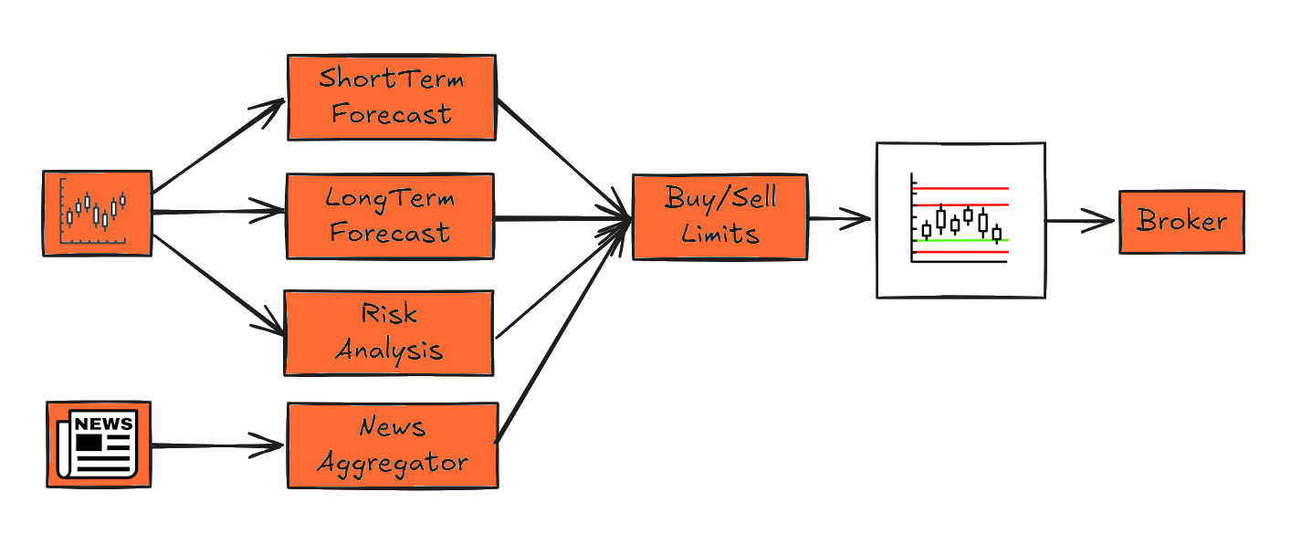
The news summarization module reads various national and international news sources. These include stock market, economic, and political news. The news is extracted from online data streams. Each news item is then processed by an AI, specifically a large language model (LLM). The AI evaluates each news item and its impact on each individual security. The resulting trend assessment indicates whether the news is expected to have a positive, negative, or neutral effect on the price of the security. News with a neutral impact is not further processed.

If a piece of news is assigned to a security and a trend has been determined, the model also evaluates whether the trend is short-term, medium-term, or long-term, as well as the relevance of the news. These KPIs are used to generate a data record. A single news item may be assigned to one or more markets, indices, or stocks. Price forecasts are based on news items stored in the database. These forecasts are available in the form of a database and are used to calculate limits for buy and sell decisions.

Collaboration with Katastrophenmelder

The professional platform katastrophenmelder.de continuously analyzes news sources. Various sources from different domains are used to detect and evaluate anomalies. A catastrophe scale is generated, drawing on topics such as weather, politics, economy, and military conflicts. The news and sources are continuously monitored. Fortunately, the system only rarely triggers an alarm. It is rare that a threshold is exceeded in such a way that the news qualifies as catastrophic. This makes the system particularly robust.

Believability/Influence Model

How to agregate sentiment data

The core idea: people tend to believe a statement when three levers align: high unique exposure, independent multi-source support, and observable evidence. Opposition reduces this effect.

Root cause of misestimation in the wild:

Reach bias: raw audience numbers are counted without removing audience overlaps.
Independence illusion: multiple outlets belong to the same owner, creating an echo that looks diversified.
Evidence neglect: narratives are amplified without checking alignment with measurable indicators.
Temporal drift: old coverage continues to influence even when outdated (insufficient decay).
Asymmetric counter-messaging: the strength and diversity of the opposing narrative is not netted out.

The model addresses these by computing effective unique exposure for supporters and opponents, weighting sources by credibility and recency, rewarding ownership diversity, applying diminishing returns for additional channels, aligning with evidence, and discounting stale signals.

Calculation

2.1 Definitions

$R s$ : reach; $A s$ : attention; $C s$ : credibility.
$x s = R s \cdotA s \cdotC s$ (raw exposure).
$D s$ (recency/decay); $x̃ s = x s \cdotD s$ .
$Ω st$ : audience overlap; $κ$ : overlap-correction strength.
Sets: supporters $P$ , opponents $Q$ .

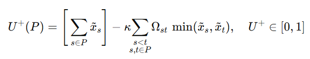
2.2 Effective Unique Exposure

The two key formulas are embedded as images to guarantee consistent rendering.

Supporters:

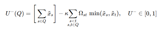
Opponents:

Difference: $ΔU = U + - U -$

2.3 Source Quality per Side

Independence (entropy-based) $D(S)$ and breadth (saturation) $B(S)$ .
Combine: $M + = λ\cdotD(P) + (1-λ)\cdotB(P)$ , $M - = λ\cdotD(Q) + (1-λ)\cdotB(Q)$
Side strengths: $S + = (U +) α \cdot(M +) ρ$ , $S - = (U -) α \cdot(M -) ρ'$

2.4 Evidence, Consistency, Recency

Evidence alignment $E$ (e.g., logistic of a standardized data agreement).
Consistency $K$ (low variance across time/channels ⇒ higher K).
Global recency $T$ from exposure-weighted mean age.
Direction factor $Φ = σ(μ\cdotΔU)$ .

2.5 Final Score

I = norm( ( S + / (1 + S -) η) \cdot E β \cdot K γ \cdot T δ \cdot Φ )

norm(z) = z / (1 + z). Choose exponents and time constants via calibration on historical outcomes.

2.6 Minimal Implementation Order

Compute $x̃ s$ with decay.
Compute $U +$ , $U -$ via overlap correction; then $ΔU$ .
Compute $D(S)$ , $B(S)$ , $M \pm$ , $S \pm$ .
Estimate $E$ , $K$ , $T$ , and $Φ$ .
Combine into $I$ and normalize.

Table of Definitions – Terms and Variables Used in the Believability/Influence Model

This table lists symbols, ranges/types, definitions, and explanations. Mathematics render via MathJax; inline math is written as $ ... $.

Symbol / Term	Range / Type	Definition	Explanation / Interpretation
$R_s$	$[0,1]$	Reach of source $s$	Fraction of the total audience exposed to source $s$ (viewership/readership share).
$A_s$	$[0,1]$	Attention weight	Prominence of placement (prime time, front page, top feed vs. low-visibility slots).
$C_s$	$[0,1]$	Credibility / reliability	Track record of accuracy and corrections for source $s$.
$x_s = R_s A_s C_s$	$[0,1]$	Weighted exposure	Raw per-source exposure prior to overlap and time decay.
$D_s$	$[0,1]$	Per-source decay	Recency weight for messages from source $s$; e.g., $D_s=\exp\!\big(-\tfrac{t_0-t_s}{\tau_x}\big)$.
$\tilde{x}_s = x_s D_s$	$[0,1]$	Time-weighted exposure	Effective exposure after applying per-source recency/decay.
$\Omega_{st}$	$[0,1]$	Audience overlap	Shared audience between sources $s$ and $t$ to correct double counting.
$\kappa$	$[0,1]$	Overlap correction strength	How strongly overlaps reduce effective unique exposure.
$g(s)$	categorical	Ownership / influence group	Organizational controller of $s$; used to compute independence.
$P$	set	Supporter sources	Set of sources propagating the target statement.
$Q$	set	Opponent sources	Set of sources countering the target statement.
$U^{+}(P)$	$[0,1]$	Effective unique exposure (supporters)	\(\displaystyle U^{+}=\sum_{s\in P}\tilde{x}_s-\kappa\!\!\sum_{\substack{s
$U^{-}(Q)$	$[0,1]$	Effective unique exposure (opponents)	\(\displaystyle U^{-}=\sum_{s\in Q}\tilde{x}_s-\kappa\!\!\sum_{\substack{s
$\Delta U$	$[-1,1]$	Exposure difference	$\Delta U=U^{+}-U^{-}$; net unique exposure advantage (sign indicates direction).
$p_G$	$[0,1]$	Group share	$\displaystyle p_G=\frac{\sum_{s\in S,\;g(s)=G}\tilde{x}_s}{\sum_{s\in S}\tilde{x}_s}$ for side $S\in\{P,Q\}$.
$H(S)$	$\ge 0$	Shannon entropy	$\displaystyle H(S)=-\sum_G p_G\log p_G$; diversity of ownership for side $S$.
$D(S)=H/\log\|G_S\|$	$[0,1]$	Normalized independence	Entropy normalized by the maximum for the number of groups; 1 = fully independent.
$B(S)=1-e^{-\sum_{s\in S}\tilde{x}_s}$	$[0,1)$	Breadth / saturation	Diminishing returns when adding more sources to side $S$.
$\lambda$	$[0,1]$	Independence–breadth balance	Convex weight between $D(S)$ and $B(S)$.
$M^{+},M^{-}$	$[0,1]$	Source quality (per side)	$M^{+}=\lambda D(P)+(1-\lambda)B(P)$, $M^{-}=\lambda D(Q)+(1-\lambda)B(Q)$.
$S^{+},S^{-}$	$[0,1]$	Side strength	$S^{+}=(U^{+})^{\alpha}(M^{+})^{\rho}$, $S^{-}=(U^{-})^{\alpha}(M^{-})^{\rho'}$.
$\Phi$	$(0,1)$	Direction factor	$\displaystyle \Phi=\sigma(\mu\,\Delta U)=\frac{1}{1+\exp(-\mu\,\Delta U)}$.
$E$	$[0,1]$	Evidence alignment	Maps standardized data agreement $z$ via $E=\sigma(\beta_z z)$.
$K$	$[0,1]$	Consistency	$\displaystyle K=1-\frac{\mathrm{Var}_w(d_{s,t})}{\mathrm{Var}_{\max}}$, weighted by time.
$T$	$[0,1]$	Global recency / freshness	$\displaystyle T=\exp\!\Big(-\frac{\bar{\tau}}{\tau_T}\Big)$, with $\bar{\tau}$ the exposure-weighted mean age.
$\tau_x,\tau_e,\tau_k,\tau_T$	positive	Time constants	Decay speeds for exposure, evidence, consistency, and global freshness.
$t_s,t_i,t_0$	timestamps	Times for messages/evidence and “now”	Inputs to decay kernels; e.g., evidence weights $w_i=\exp(-\tfrac{t_0-t_i}{\tau_e})$.
$d$	$\{-1,0,1\}$	Stated direction	Polarity of the claim (e.g., “increase”, “neutral”, “decrease”).
$\Delta y$	real	Observed change	Measured indicator change used to compute evidence alignment.
$z$	real	Evidence z-score	Standardized alignment of $d$ and $\Delta y$ over a window.
$\alpha,\beta,\gamma,\delta,\eta,\rho,\rho'$	positive	Model exponents	Control sensitivity to side strength, evidence, consistency, freshness, and opposition.
$\mu$	positive	Direction sensitivity	Steepness of logistic mapping from $\Delta U$ to $\Phi$.
$\sigma(x)$	function	Logistic sigmoid	$\sigma(x)=\dfrac{1}{1+\exp(-x)}$; used for $E$ and $\Phi$.
$\mathrm{norm}(z)$	function	Score normalization	Bounds output to $[0,1]$, commonly $\mathrm{norm}(z)=\dfrac{z}{1+z}$.
$I$	$[0,1]$	Believability / influence score	Final bounded score of the model.

Comprehensive Believability/Influence Model

Step	Mathematical Expression	Description / Purpose
Per-source Recency / Decay	\[ d_{\exp}(t_s) = e^{-\frac{t_0 - t_s}{\tau_x}} \] \[ d_{\text{pl}}(t_s) = \left(1 + \frac{t_0 - t_s}{\tau_p}\right)^{-\zeta} \] \[ D_s = \omega\, d_{\exp}(t_s) + (1-\omega)\, d_{\text{pl}}(t_s) \] \[ \tilde{x}_s = x_s\,D_s \]	Older messages weigh less; $\tilde{x}_s$ is exposure after time decay.
Effective Unique Exposure	Supporters: Opponents: Difference: \[ \Delta U \;=\; U^{+} \;-\; U^{-} \]	Overlap correction removes double counting before comparing sides.
Independence & Breadth	\[ p_G = \frac{\sum_{s \in S,\, g(s)=G}\tilde{x}_s}{\sum_{s \in S}\tilde{x}_s},\quad H(S) = -\sum_G p_G \log p_G \] \[ D(S) = \frac{H(S)}{\log \|G_S\|}, \quad B(S) = 1 - e^{-\sum_{s \in S}\tilde{x}_s} \] \[ M^{+} = \lambda D(P) + (1-\lambda)B(P), \quad M^{-} = \lambda D(Q) + (1-\lambda)B(Q) \]	Entropy-based independence plus saturation-based breadth form side quality.
Evidence & Consistency	\[ z = \frac{\mathbb{E}[d\,\Delta y]}{\sigma_{\Delta y}}, \quad E = \sigma(\beta_z z) = \frac{1}{1+e^{-\beta_z z}} \] \[ K = 1 - \frac{\mathrm{Var}_w(d_{s,t})}{\mathrm{Var}_{\max}}, \quad w_i = e^{-\frac{t_0 - t_i}{\tau_e}} \]	Data agreement and message stability, both time-weighted.
Side Strength & Direction	\[ S^{+} = (U^{+})^{\alpha}(M^{+})^{\rho}, \quad S^{-} = (U^{-})^{\alpha}(M^{-})^{\rho'} \] \[ \Phi = \sigma(\mu\,\Delta U) = \frac{1}{1 + e^{-\mu\,\Delta U}} \]	Strength per side; $\Phi$ biases toward the dominant exposure.
Global Recency	\[ \bar{\tau} = \frac{\sum_{s \in P \cup Q}\tilde{x}_s\,(t_0 - t_s)}{\sum_{s \in P \cup Q}\tilde{x}_s} \] \[ T = e^{-\frac{\bar{\tau}}{\tau_T}} \]	Overall freshness penalty when discourse is stale.
Comprehensive Score	\[ I = \mathrm{norm}\!\left( \frac{S^{+}}{(1+S^{-})^{\eta}} \cdot E^{\beta} \cdot K^{\gamma} \cdot T^{\delta} \cdot \Phi \right), \quad \mathrm{norm}(z)=\frac{z}{1+z} \]	Final bounded believability score $I \in [0,1]$.

Anomaly Detection

The module for detecting price anomalies

The anomaly detection module analyzes price behavior in order to identify sudden spikes—either upward or downward. Over a longer time period, it determines the typical range in which a security moves. Significant deviations above or below this range are detected and trigger an alert. Alerts from Katastrophenmelder and the anomaly detection module are manually reviewed and incorporated into the buy decision process.

News Processing System

Our advanced news processing system categorizes and analyzes information from multiple sources to provide actionable trading insights.

📰

News Collection

Gathering data from diverse global sources

🔍

Analysis

AI-powered evaluation of news impact

📊

Trend Assessment

Determining positive, negative, or neutral effects

⏱️

Time Classification

Categorizing as short, medium, or long-term impacts

Symbol / Term	Range / Type	Definition	Explanation / Interpretation
\(R_s\)	\([0,1]\)	Reach of source \(s\)	Fraction of the total audience exposed to source \(s\) (viewership/readership share).
\(A_s\)	\([0,1]\)	Attention weight	Prominence of placement (prime time, front page, top feed vs. low-visibility slots).
\(C_s\)	\([0,1]\)	Credibility / reliability	Track record of accuracy and corrections for source \(s\).
\(x_s = R_s A_s C_s\)	\([0,1]\)	Weighted exposure	Raw per-source exposure prior to overlap and time decay.
\(D_s\)	\([0,1]\)	Per-source decay	Recency weight for messages from source \(s\); e.g., \(D_s=\exp\!\big(-\tfrac{t_0-t_s}{\tau_x}\big)\).
\(\tilde{x}_s = x_s D_s\)	\([0,1]\)	Time-weighted exposure	Effective exposure after applying per-source recency/decay.
\(\Omega_{st}\)	\([0,1]\)	Audience overlap	Shared audience between sources \(s\) and \(t\) to correct double counting.
\(\kappa\)	\([0,1]\)	Overlap correction strength	How strongly overlaps reduce effective unique exposure.
\(g(s)\)	categorical	Ownership / influence group	Organizational controller of \(s\); used to compute independence.
\(P\)	set	Supporter sources	Set of sources propagating the target statement.
\(Q\)	set	Opponent sources	Set of sources countering the target statement.
\(U^{+}(P)\)	\([0,1]\)	Effective unique exposure (supporters)	\(\displaystyle U^{+}=\sum_{s\in P}\tilde{x}_s-\kappa\!\!\sum_{\substack{s
\(U^{-}(Q)\)	\([0,1]\)	Effective unique exposure (opponents)	\(\displaystyle U^{-}=\sum_{s\in Q}\tilde{x}_s-\kappa\!\!\sum_{\substack{s
\(\Delta U\)	\([-1,1]\)	Exposure difference	\(\Delta U=U^{+}-U^{-}\); net unique exposure advantage (sign indicates direction).
\(p_G\)	\([0,1]\)	Group share	\(\displaystyle p_G=\frac{\sum_{s\in S,\;g(s)=G}\tilde{x}_s}{\sum_{s\in S}\tilde{x}_s}\) for side \(S\in\{P,Q\}\).
\(H(S)\)	\(\ge 0\)	Shannon entropy	\(\displaystyle H(S)=-\sum_G p_G\log p_G\); diversity of ownership for side \(S\).
\(D(S)=H/\log\|G_S\|\)	\([0,1]\)	Normalized independence	Entropy normalized by the maximum for the number of groups; 1 = fully independent.
\(B(S)=1-e^{-\sum_{s\in S}\tilde{x}_s}\)	\([0,1)\)	Breadth / saturation	Diminishing returns when adding more sources to side \(S\).
\(\lambda\)	\([0,1]\)	Independence–breadth balance	Convex weight between \(D(S)\) and \(B(S)\).
\(M^{+},M^{-}\)	\([0,1]\)	Source quality (per side)	\(M^{+}=\lambda D(P)+(1-\lambda)B(P)\), \(M^{-}=\lambda D(Q)+(1-\lambda)B(Q)\).
\(S^{+},S^{-}\)	\([0,1]\)	Side strength	\(S^{+}=(U^{+})^{\alpha}(M^{+})^{\rho}\), \(S^{-}=(U^{-})^{\alpha}(M^{-})^{\rho'}\).
\(\Phi\)	\((0,1)\)	Direction factor	\(\displaystyle \Phi=\sigma(\mu\,\Delta U)=\frac{1}{1+\exp(-\mu\,\Delta U)}\).
\(E\)	\([0,1]\)	Evidence alignment	Maps standardized data agreement \(z\) via \(E=\sigma(\beta_z z)\).
\(K\)	\([0,1]\)	Consistency	\(\displaystyle K=1-\frac{\mathrm{Var}_w(d_{s,t})}{\mathrm{Var}_{\max}}\), weighted by time.
\(T\)	\([0,1]\)	Global recency / freshness	\(\displaystyle T=\exp\!\Big(-\frac{\bar{\tau}}{\tau_T}\Big)\), with \(\bar{\tau}\) the exposure-weighted mean age.
\(\tau_x,\tau_e,\tau_k,\tau_T\)	positive	Time constants	Decay speeds for exposure, evidence, consistency, and global freshness.
\(t_s,t_i,t_0\)	timestamps	Times for messages/evidence and “now”	Inputs to decay kernels; e.g., evidence weights \(w_i=\exp(-\tfrac{t_0-t_i}{\tau_e})\).
\(d\)	\(\{-1,0,1\}\)	Stated direction	Polarity of the claim (e.g., “increase”, “neutral”, “decrease”).
\(\Delta y\)	real	Observed change	Measured indicator change used to compute evidence alignment.
\(z\)	real	Evidence z-score	Standardized alignment of \(d\) and \(\Delta y\) over a window.
\(\alpha,\beta,\gamma,\delta,\eta,\rho,\rho'\)	positive	Model exponents	Control sensitivity to side strength, evidence, consistency, freshness, and opposition.
\(\mu\)	positive	Direction sensitivity	Steepness of logistic mapping from \(\Delta U\) to \(\Phi\).
\(\sigma(x)\)	function	Logistic sigmoid	\(\sigma(x)=\dfrac{1}{1+\exp(-x)}\); used for \(E\) and \(\Phi\).
\(\mathrm{norm}(z)\)	function	Score normalization	Bounds output to \([0,1]\), commonly \(\mathrm{norm}(z)=\dfrac{z}{1+z}\).
\(I\)	\([0,1]\)	Believability / influence score	Final bounded score of the model.

Step	Mathematical Expression	Description / Purpose
Per-source Recency / Decay	\[ d_{\exp}(t_s) = e^{-\frac{t_0 - t_s}{\tau_x}} \] \[ d_{\text{pl}}(t_s) = \left(1 + \frac{t_0 - t_s}{\tau_p}\right)^{-\zeta} \] \[ D_s = \omega\, d_{\exp}(t_s) + (1-\omega)\, d_{\text{pl}}(t_s) \] \[ \tilde{x}_s = x_s\,D_s \]	Older messages weigh less; \(\tilde{x}_s\) is exposure after time decay.
Effective Unique Exposure	Supporters: Opponents: Difference: \[ \Delta U \;=\; U^{+} \;-\; U^{-} \]	Overlap correction removes double counting before comparing sides.
Independence & Breadth	\[ p_G = \frac{\sum_{s \in S,\, g(s)=G}\tilde{x}_s}{\sum_{s \in S}\tilde{x}_s},\quad H(S) = -\sum_G p_G \log p_G \] \[ D(S) = \frac{H(S)}{\log \|G_S\|}, \quad B(S) = 1 - e^{-\sum_{s \in S}\tilde{x}_s} \] \[ M^{+} = \lambda D(P) + (1-\lambda)B(P), \quad M^{-} = \lambda D(Q) + (1-\lambda)B(Q) \]	Entropy-based independence plus saturation-based breadth form side quality.
Evidence & Consistency	\[ z = \frac{\mathbb{E}[d\,\Delta y]}{\sigma_{\Delta y}}, \quad E = \sigma(\beta_z z) = \frac{1}{1+e^{-\beta_z z}} \] \[ K = 1 - \frac{\mathrm{Var}_w(d_{s,t})}{\mathrm{Var}_{\max}}, \quad w_i = e^{-\frac{t_0 - t_i}{\tau_e}} \]	Data agreement and message stability, both time-weighted.
Side Strength & Direction	\[ S^{+} = (U^{+})^{\alpha}(M^{+})^{\rho}, \quad S^{-} = (U^{-})^{\alpha}(M^{-})^{\rho'} \] \[ \Phi = \sigma(\mu\,\Delta U) = \frac{1}{1 + e^{-\mu\,\Delta U}} \]	Strength per side; \(\Phi\) biases toward the dominant exposure.
Global Recency	\[ \bar{\tau} = \frac{\sum_{s \in P \cup Q}\tilde{x}_s\,(t_0 - t_s)}{\sum_{s \in P \cup Q}\tilde{x}_s} \] \[ T = e^{-\frac{\bar{\tau}}{\tau_T}} \]	Overall freshness penalty when discourse is stale.
Comprehensive Score	\[ I = \mathrm{norm}\!\left( \frac{S^{+}}{(1+S^{-})^{\eta}} \cdot E^{\beta} \cdot K^{\gamma} \cdot T^{\delta} \cdot \Phi \right), \quad \mathrm{norm}(z)=\frac{z}{1+z} \]	Final bounded believability score \(I \in [0,1]\).